FIERY论文与代码解读,LSS原理与代码解读
FIERY整体结构
FIERY是时序的实例分割和预测网络,在不依赖高清地图的情况下,仅从摄像头驱动数据中以端到端的方式学习对未来固有的随机性进行建模,并预测未来的多时间轨迹。效果可视化如下图所示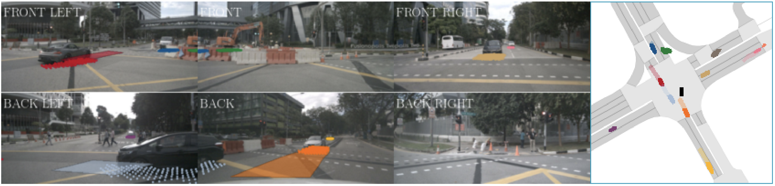
FIERY的整体结构如下图所示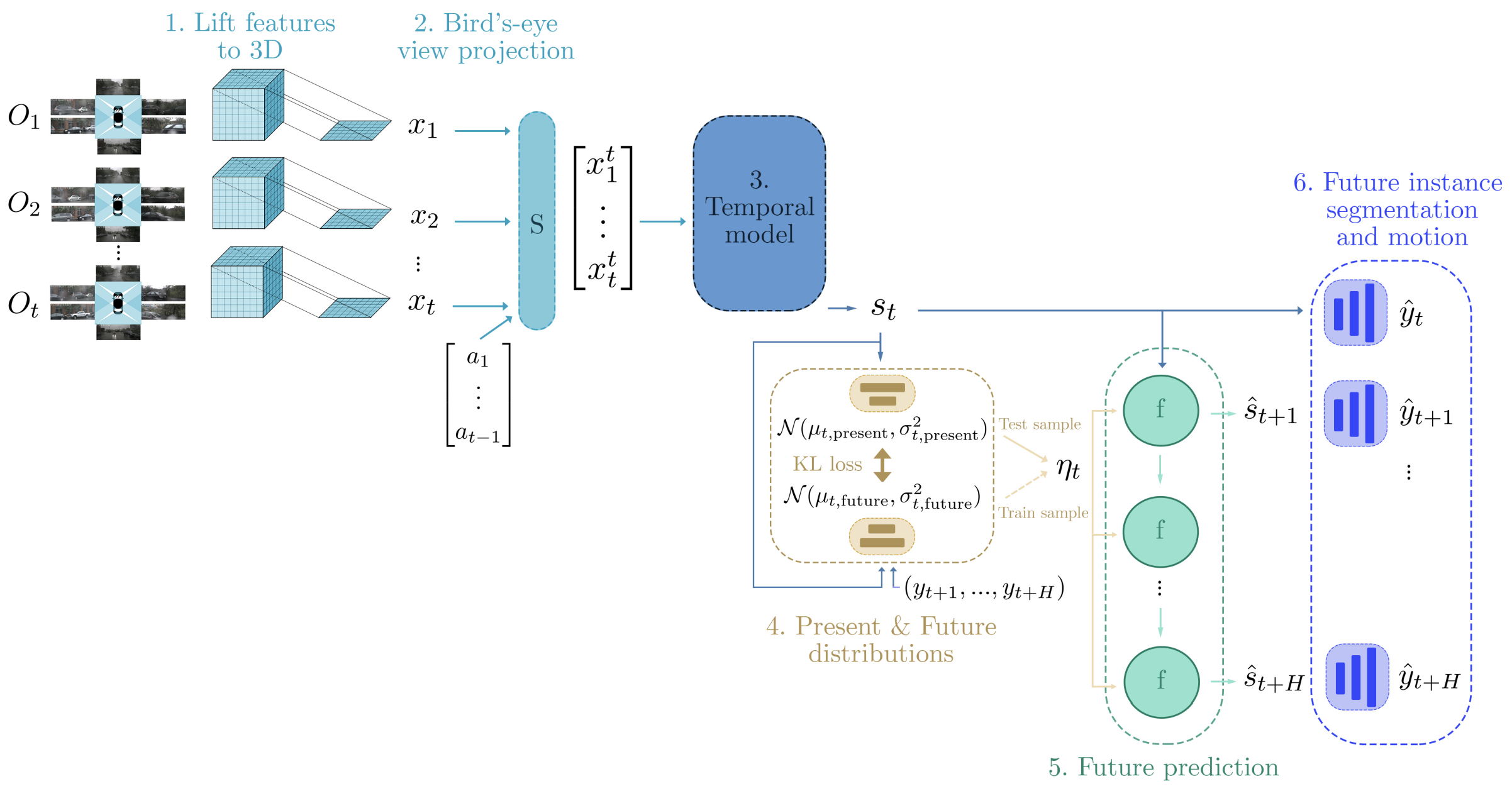
FIERY的整体结构可以分为6个部分。
- 根据相机的内外参和估计的深度概率分布,将图像特征转为3D特征
- 将上述得到的各个视角的3D特征,投影到BEV空间,然后基于惯导提供的运动信息,将过去两帧的BEV特征与当前帧的BEV特征对齐
- 使用一个基于3D卷积的时序模块学习时空状态${s_t}$
- 参数化两个概率分布,分别为当前分布 和 未来分布。当前分布以当前的时空状态$s_t$为条件,未来分布则同时以当前的时空状态$s_t$和未来的标签${(y_{t+1}, …, y_{t+H})}$为条件
- 我们在训练过程中从未来分布中采样潜在编码$\eta_t$,而在推理期间从当前分布中采样。当前状态$s_t$和潜在编码$\eta_t$是未来预测模型的输入,它递归地预测未来的状态${(\hat{s}_{t+1}, …, \hat{s}_{t+H})}$。
- 这些状态被解码为BEV视角的未来实例分割和未来的运动
经过一系列编解码,最终得到的结果如下图所示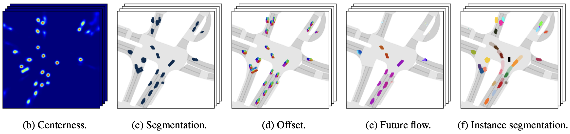
各模块具体的实现原理将拆解成单独的几部分进行介绍。
LSS (ECCV 2020)
FIERY从2D特征到3D BEV特征的转换过程采用的是LSS的方式(以下具体介绍部分还是以FIERY的设定为例,避免混淆)。LSS是NVIDIA在2020年提出的方案,是自动驾驶多目相机感知领域的非常重要的论文。其最大的贡献在于:提供了一个端到端的训练方法解决多个传感器融合的问题。传统的多个传感器单独检测后再进行后处理的方法无法将此过程损失传进行反向传播而调整相机输入,而LSS则省去了这一阶段的后处理,直接输出融合结果。
LSS分别对应Lift, Splat, Shoot三个步骤。原文中对其解释如下
The core idea behind our approach is to “lift” each image individually into a frustum of features for each camera, then “splat” all frustums into a rasterized bird’s-eyeview grid.
…
The representations inferred by our model enable interpretable end-to-end motion planning by “shooting” template trajectories into a bird’s-eyeview cost map output by our network.
Lift
该步骤是将每个图像单独“lift”为每个相机的特征截锥体,该过程的可视化如下图所示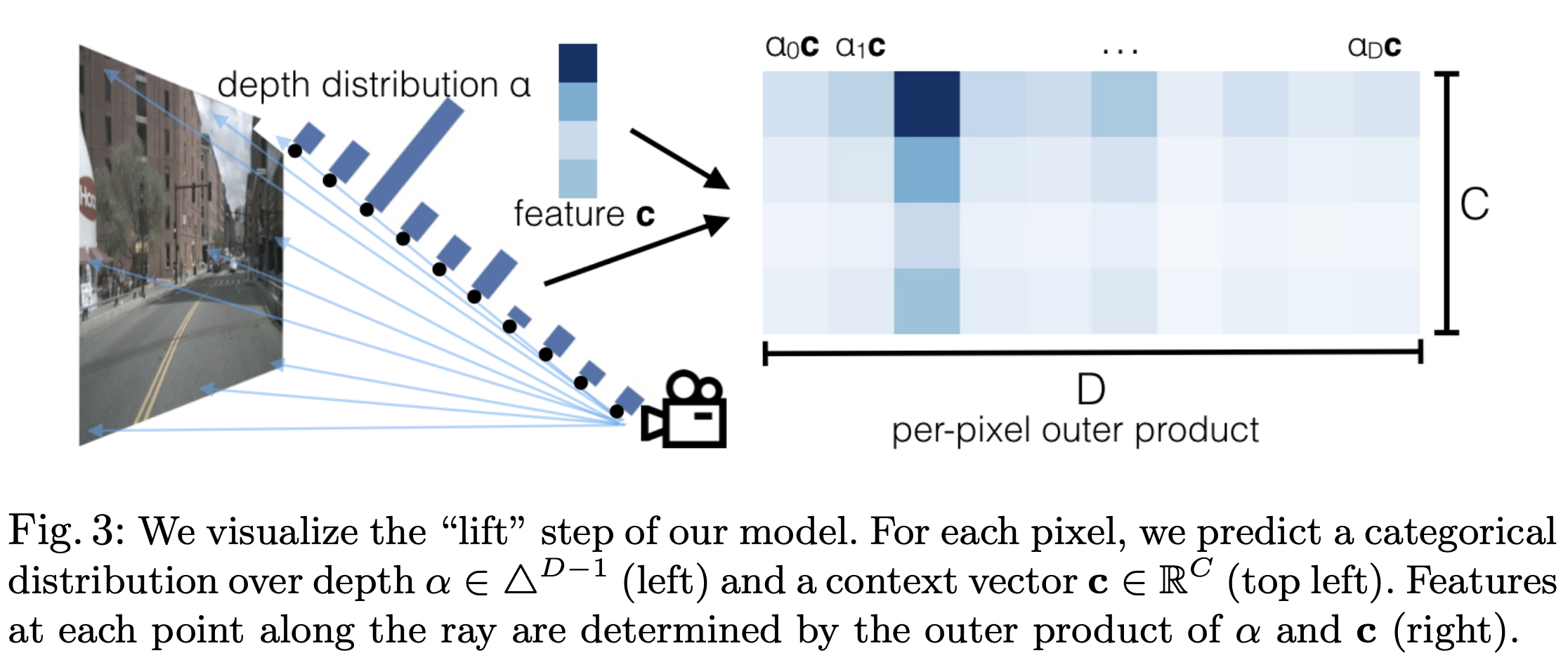
根据相机的成像原理,每个像素实际上是空间中的一条射线经过相机中心在像平面上的投影。因此,对于每个像素,在已知相机的内外参的情况下,我们只能确定这条射线,但不能确定这个像素具体反映的是射线上哪个点的信息,也就是常说的depth。因此,LSS预先设定了相机的视锥,深度方向的范围是${[d_{min}, d_{max}]}$。在FIERY的实现版本中,深度范围是${[2, 50)}$,每隔1米进行采样,因此可以得到48个离散的深度值。在这个范围内进行概率估计,然后将深度概率估计与图像特征进行内积,从而能够得到每个相机视锥体。该部分的Tensor变换如下图所示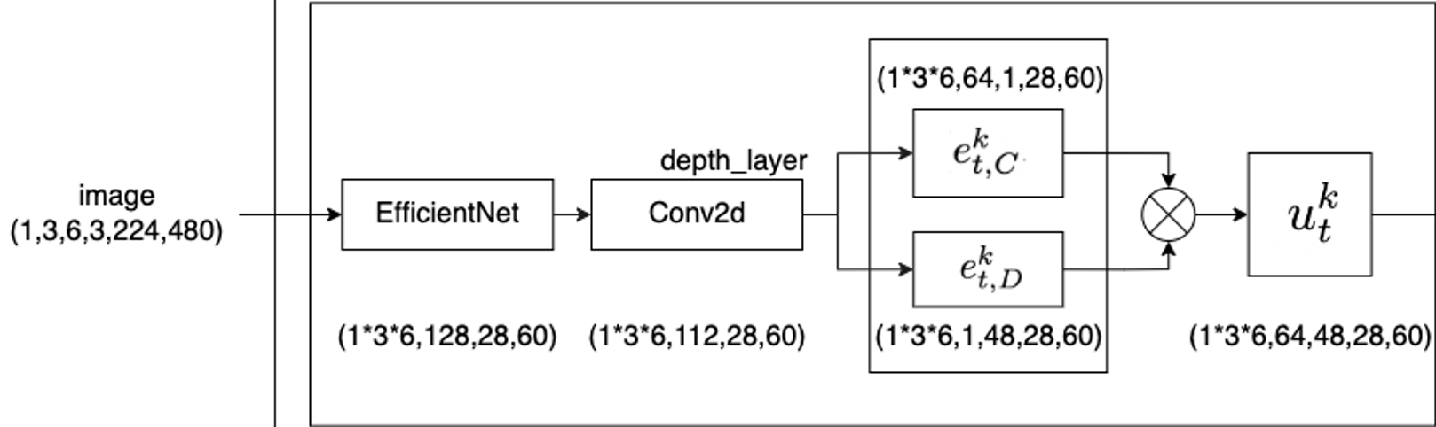
在实现方面,实际上就直接使用卷积层实现。softmax之后得到深度估计的概率分布,然后将其与特征做外积,具体代码如下,
class Encoder(nn.Module):
    def __init__(self, cfg, D):
        super().__init__()
        self.D = D
        self.C = cfg.OUT_CHANNELS
        # ...

    def forward(self, x):
        x = self.depth_layer(x)  # feature and depth head
        if self.use_depth_distribution:
            depth = x[:, : self.D].softmax(dim=1)
            x = depth.unsqueeze(1) * x[:, self.D : (self.D + self.C)].unsqueeze(2)  # outer product depth and features
        else:
            x = x.unsqueeze(2).repeat(1, 1, self.D, 1, 1)
        return x
Splat
Splat步骤是将各个相机的视锥体投影到BEV视角。该部分的Tensor变换如下图所示
要实现这个投影,就要得到相机视锥体到BEV空间的坐标转换关系。此处首先依赖相机的内外参生成一个Geometry,它用于存储每个相机视锥体的各个特征到整体3D空间(后续会降维到BEV空间)的对应关系。首先,初始化一个$D\times W \times H$ 的frustum。按照图像坐标系 -> 归一化相机坐标系 -> 相机坐标系 -> 车身坐标系的坐标转换顺序计算得到对应坐标。该部分代码实现如下(其中涉及到的坐标转换部分,可以参考这篇自动驾驶中的常见坐标转换与Nuscenes中的坐标转换实战)
def get_geometry(self, intrinsics, extrinsics):
    """
    Calculate the (x, y, z) 3D position of the features.
    """
    rotation, translation = extrinsics[..., :3, :3], extrinsics[..., :3, 3]
    B, N, _ = translation.shape
    # Add batch, camera dimension, and a dummy dimension at the end
    # self.frustum是预定义的相机视锥体的三维网格
    points = self.frustum.unsqueeze(0).unsqueeze(0).unsqueeze(-1)

    # Camera to ego reference frame
    # 反归一化
    points = torch.cat((points[:, :, :, :, :, :2] * points[:, :, :, :, :, 2:3], points[:, :, :, :, :, 2:3]), 5)
    combined_transformation = rotation.matmul(torch.inverse(intrinsics))
    points = combined_transformation.view(B, N, 1, 1, 1, 3, 3).matmul(points).squeeze(-1)
    points += translation.view(B, N, 1, 1, 1, 3)

    # The 3 dimensions in the ego reference frame are: (forward, sides, height)
    return points
得到Geometry之后,就可以利用Voxel Pooling构建BEV特征。具体来说,将相机点云投影到预先划定范围的3D空间中。此时,可能会有多个视觉特征对应同一个BEV网格,直接将能投影到同一个BEV网格的特征累加起来,就可以得到降维后的BEV特征。该部分代码实现如下
def projection_to_birds_eye_view(self, x, geometry):
    # batch, n_cameras, depth, height, width, channels
    batch, n, d, h, w, c = x.shape
    output = torch.zeros(
        (batch, c, self.bev_dimension[0], self.bev_dimension[1]), dtype=torch.float, device=x.device
    )

    # Number of 3D points
    N = n * d * h * w
    for b in range(batch):
        # 展平视觉点云
        x_b = x[b].reshape(N, c)

        # 计算栅格坐标并取整
        geometry_b = ((geometry[b] - (self.bev_start_position - self.bev_resolution / 2.0)) / self.bev_resolution)
        # 展平体素坐标
        geometry_b = geometry_b.view(N, 3).long()

        # Mask out points that are outside the considered spatial extent.
        mask = (
                (geometry_b[:, 0] >= 0)
                & (geometry_b[:, 0] < self.bev_dimension[0])
                & (geometry_b[:, 1] >= 0)
                & (geometry_b[:, 1] < self.bev_dimension[1])
                & (geometry_b[:, 2] >= 0)
                & (geometry_b[:, 2] < self.bev_dimension[2])
        )
        x_b = x_b[mask]
        geometry_b = geometry_b[mask]

        # Sort tensors so that those within the same voxel are consecutives.
        ranks = (
                geometry_b[:, 0] * (self.bev_dimension[1] * self.bev_dimension[2])
                + geometry_b[:, 1] * (self.bev_dimension[2])
                + geometry_b[:, 2]
        )
        ranks_indices = ranks.argsort()
        x_b, geometry_b, ranks = x_b[ranks_indices], geometry_b[ranks_indices], ranks[ranks_indices]

        # Project to bird's-eye view by summing voxels.
        x_b, geometry_b = VoxelsSumming.apply(x_b, geometry_b, ranks)

        bev_feature = torch.zeros((self.bev_dimension[2], self.bev_dimension[0], self.bev_dimension[1], c),
                                    device=x_b.device)
        bev_feature[geometry_b[:, 2], geometry_b[:, 0], geometry_b[:, 1]] = x_b

        # Put channel in second position and remove z dimension
        bev_feature = bev_feature.permute((0, 3, 1, 2))
        bev_feature = bev_feature.squeeze(0)

        output[b] = bev_feature

    return output
时序特征对齐
经过上一步,我们已经得到多帧的BEV特征。由于车辆的运动,每一帧的BEV特征可能都处于不同的位置,因此需要将过去时刻的BEV特征warp到当前时刻以统一坐标系,也就是所谓的特征对齐(feature alignment)。这个步骤基本就是简单的坐标系转换,借助惯导信息来完成。该部分的Tensor变换如下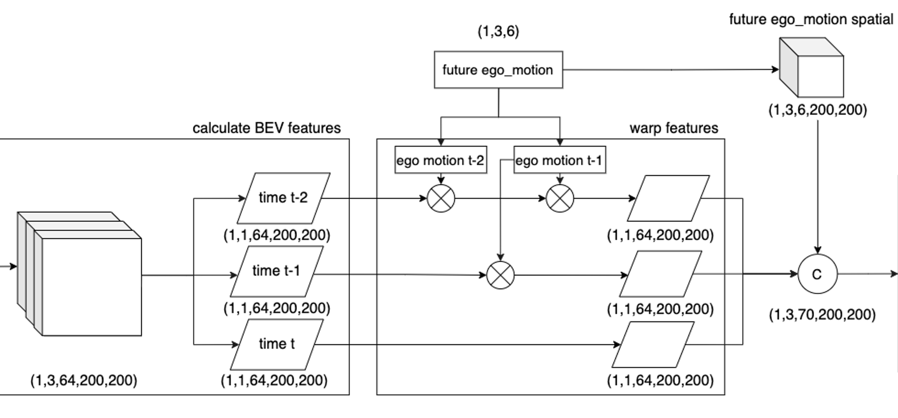
惯导提供的信息通常是相对于起始位置的三轴平移量和三轴旋转量。根据两帧的惯导数据,可以很容易的计算出两帧之间的相对平移量和旋转量,即$[tx, ty, tz, rx, ry, rz]$。然后,基于这个运动信息,实现feature warp(由于涉及到连续多帧的变换,会先将这个6 DoF转成坐标转换矩阵的形式,然后再转回6 DoF的形式)。先进行Z轴上的旋转,然后进行X轴、Y轴的平移,最后使用仿射变换实现X轴、Y轴的旋转。
def warp_features(x, flow, mode='nearest', spatial_extent=None):
    """ Applies a rotation and translation to feature map x.
        Args:
            x: (b, c, h, w) feature map
            flow: (b, 6) 6DoF vector (only uses the xy poriton)
            mode: use 'nearest' when dealing with categorical inputs
        Returns:
            in plane transformed feature map
        """
    if flow is None:
        return x
    b, c, h, w = x.shape
    # z-rotation
    angle = flow[:, 5].clone()  # torch.atan2(flow[:, 1, 0], flow[:, 0, 0])
    # x-y translation
    translation = flow[:, :2].clone()  # flow[:, :2, 3]

    # Normalise translation. Need to divide by how many meters is half of the image.
    # because translation of 1.0 correspond to translation of half of the image.
    translation[:, 0] /= spatial_extent[0]
    translation[:, 1] /= spatial_extent[1]
    # forward axis is inverted
    translation[:, 0] *= -1

    cos_theta = torch.cos(angle)
    sin_theta = torch.sin(angle)

    # output = Rot.input + translation
    # tx and ty are inverted as is the case when going from real coordinates to numpy coordinates
    # translation_pos_0 -> positive value makes the image move to the left
    # translation_pos_1 -> positive value makes the image move to the top
    # Angle -> positive value in rad makes the image move in the trigonometric way
    transformation = torch.stack([cos_theta, -sin_theta, translation[:, 1],
                                  sin_theta, cos_theta, translation[:, 0]], dim=-1).view(b, 2, 3)

    # Note that a rotation will preserve distances only if height = width. Otherwise there's
    # resizing going on. e.g. rotation of pi/2 of a 100x200 image will make what's in the center of the image
    grid = torch.nn.functional.affine_grid(transformation, size=x.shape, align_corners=False)
    warped_x = torch.nn.functional.grid_sample(x, grid.float(), mode=mode, padding_mode='zeros', align_corners=False)

    return warped_x

def cumulative_warp_features(x, flow, mode='nearest', spatial_extent=None):
    """ Warps a sequence of feature maps by accumulating incremental 2d flow.
    x[:, -1] remains unchanged
    x[:, -2] is warped using flow[:, -2]
    x[:, -3] is warped using flow[:, -3] @ flow[:, -2]
    ...
    x[:, 0] is warped using flow[:, 0] @ ... @ flow[:, -3] @ flow[:, -2]
    Args:
        x: (b, t, c, h, w) sequence of feature maps
        flow: (b, t, 6) sequence of 6 DoF pose
            from t to t+1 (only uses the xy poriton)

    """
    sequence_length = x.shape[1]
    if sequence_length == 1:
        return x

    # Convert 6DoF parameters to transformation matrix.
    flow = pose_vec2mat(flow)

    out = [x[:, -1]]
    cum_flow = flow[:, -2]
    for t in reversed(range(sequence_length - 1)):
        out.append(warp_features(x[:, t], mat2pose_vec(cum_flow), mode=mode, spatial_extent=spatial_extent))
        # @ is the equivalent of torch.bmm
        cum_flow = flow[:, t - 1] @ cum_flow

    return torch.stack(out[::-1], 1)
时序模块
在送入时序模块之前,FIERY将过去时刻的运动信息拓展维度之后与上一步中得到的对齐之后的BEV特征concate起来,作为时序模块的输入。时序模块实际上是一个带有局部时空卷积和全局3D池化的3D卷积网络。该模块的Tensor变换如下图所示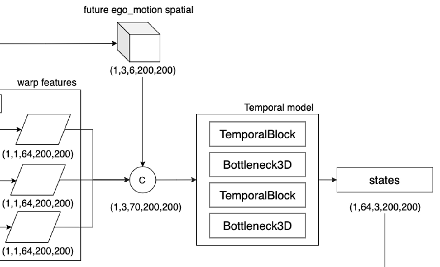
这部分的代码就不做展开了,主要就是时序block和bottleneck3D block的叠加。
当前/未来分布估计模块
这歌步骤是采用条件变分方法对未来预测的固有随机性进行建模。当前分布和未来分布都被参数化为对角高斯(diagonal Gaussians)。然后使用一个KL散度的loss来监督分布的学习。这一部分的Tensor变换如下图所示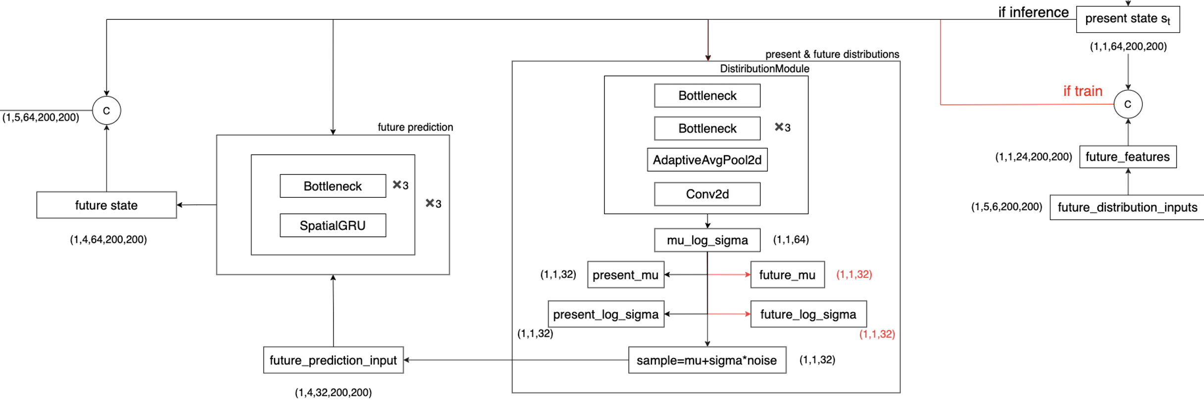
具体的代码实现如下
if self.n_future > 0:
    present_state = states[:, :1].contiguous()
    if self.cfg.PROBABILISTIC.ENABLED:
        # Do probabilistic computation
        sample, output_distribution = self.distribution_forward(
            present_state, future_distribution_inputs, noise
        )
        output = {**output, **output_distribution}

    # Prepare future prediction input
    b, _, _, h, w = present_state.shape
    hidden_state = present_state[:, 0]

    if self.cfg.PROBABILISTIC.ENABLED:
        future_prediction_input = sample.expand(-1, self.n_future, -1, -1, -1)
    else:
        future_prediction_input = hidden_state.new_zeros(b, self.n_future, self.latent_dim, h, w)

    # Recursively predict future states
    future_states = self.future_prediction(future_prediction_input, hidden_state)

    # Concatenate present state
    future_states = torch.cat([present_state, future_states], dim=1)
实例分割和运动预测
这部分是模型的Decoder部分,包括语义分割、实例中心点、实例偏移和未来实例流在内的多个head。该部分的Tensor变换如下图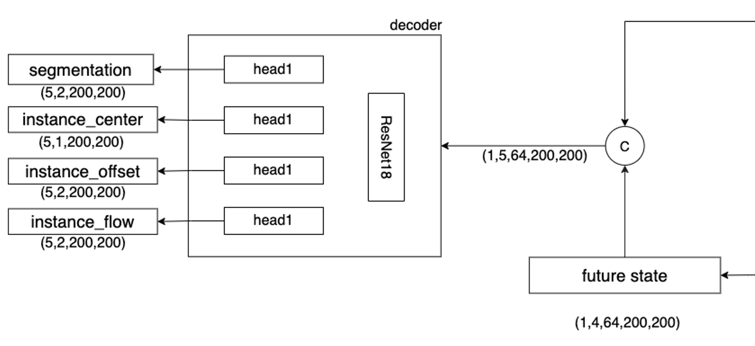
这些head都是由两层卷积得到结果,具体代码也不做展开。多个输出结果融合得到最后的轨迹可视化,这些部分都在后处理中进行。本博客在FIERY后处理原理与代码解读 中对FIERY的后处理部分进行了详细的讲解,并开源了Fiery后处理的代码(C++版),有兴趣的读者可以参考GitHub仓库。
FIERY Loss
distribution
During training, we use samples $\eta_t \sim N(\mu_{t, future}, \sigma^2_{t, future})$ from the future distribution to enforce predictions consistent with the observed future, and a mode covering Kullback-Leibler divergence loss to encourage the present distribution to cover the observed futures:
对于分布估计,使用的是KL散度进行监督。KL散度可以用来衡量两个概率分布之间的相似性,两个概率分布越相近,KL散度越小。论文中将present distribution和future distribution都参数化为均值为$\mu$,方差为$\sigma^2$的对角高斯。在loss中,KL散度的定义具体表示为
KL散度损失的具体定义可以参考BEV模型常用LOSS总结
segmentation
For semantic segmentation, we use a top-k cross-entropy loss. As the bird’s-eye view image is largely dominated by the background, we only backpropagate the top-k hardest pixels.
对于语义分割的结果,使用的是cross-entropy进行监督。交叉熵主要刻画的是实际输出(概率)与期望输出(概率)的距离,也就是交叉熵的值越小,两个概率分布就越接近。此外,原文提到只对top-k个像素进行,因为针对整个BEV Tensor进行的分类监督,背景占绝大多数,loss较小可认为学会了,既然学会了就没有必要再学,也就不需要bp了。top-k 定义的比例是25%。交叉熵损失的具体定义可以参考BEV模型常用LOSS总结
centerness
对于中心点回归,使用的是 l2 loss
offset & flow
offset和flow的回归都使用的l1 loss
FIERY 指标
针对语义分割结果的指标使用的是IoU(阈值为0.5)。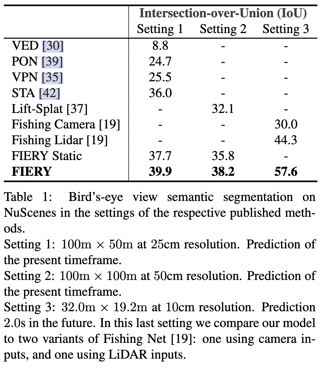
针对时序分割的指标使用的是FIERY自己定义的VPQ(Video Panoptic Quality),具体来说这个指标希望能够衡量识别质量RQ和分割质量SQ方面的性能,其中
RQ:衡量随着时间的推移,实例被检测到的一致性
SQ:实例分割的准确性
VPQ的定义如下
此处对于真正例的定义是1.IoU超过0.5;2.实例id在不同时刻保持一致
FIERY缺点
- 在网络架构中,没有进行帧间的跟踪,是在后处理过程中经过匈牙利匹配得到的;
- 非常耗时,3帧处理,加速后在orin平台部署也只能达到11hz;
- 强依赖精准内外参,行车过程中的参数变化会对结果产生比较大的影响。
参考
Fiery Paper
LSS Paper
https://developer.aliyun.com/article/1173815
https://zhuanlan.zhihu.com/p/589146284
https://pytorch.org/docs/stable/generated/torch.nn.KLDivLoss.html
https://pytorch.org/docs/stable/generated/torch.nn.CrossEntropyLoss.html